# Background

The DANA paper is a pretty cool idea which I came across recently. Its goal is to facilitate the understanding of a netlist of logic-gates, making abstractions out of Flip-Flops (FF) into higher level registers so that the flow of data can be better understood.

Before I start explaning the idea, I want to make sure we understand what these things even mean. A flip-flop is a logic gate that looks like this: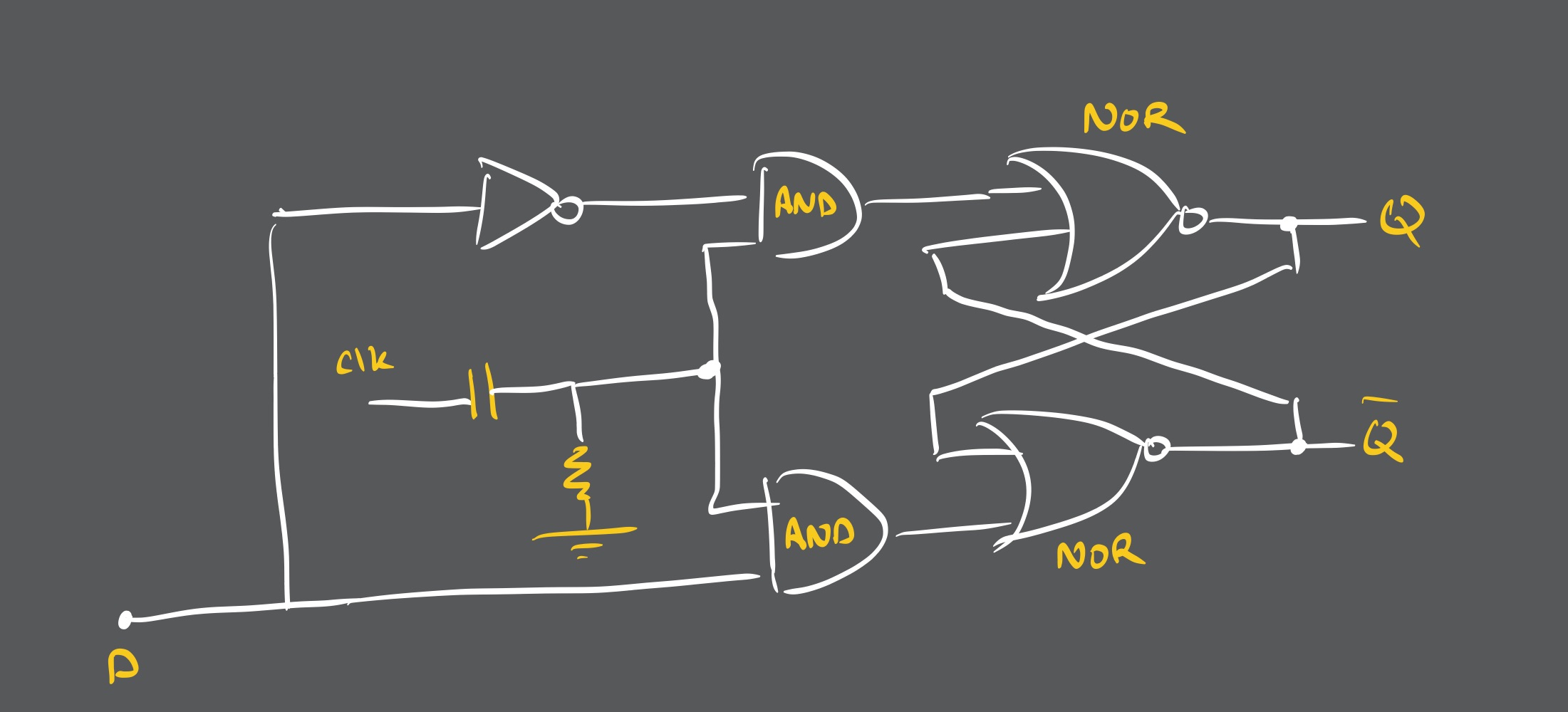

It a modification of a latch, that is the right hand part of the circuit with the NOR gates cross linked together. The outputs come as Q and ~Q and a single input D drives it. The capacitor and resistor in the middle is to convert the clock signal to a pulse which rises with the edge and quickly dies down. This gives enough time for the Q state to reflect whatever D was when the clock pulse was recieved.

In other words, its a 1-bit storage with stores a new value (or retains the old one) every clock pulse. If you’re working with an ASIC or some design involving FSMs (Finite-State-Machines) then you will use FFs to either store the state or combine together to form registers.

What about netlists? If we open one up on HAL (A framework for reverse-engineering of ASICs):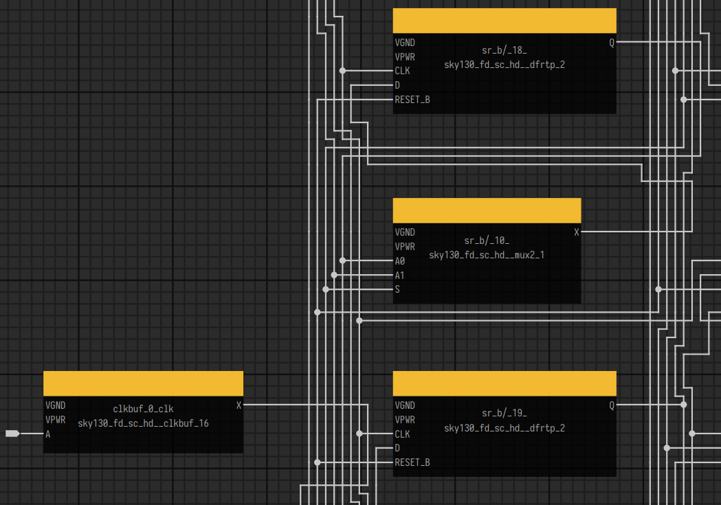

Its a mess that looks like this, on a very very large scale (imagine millions of these boxes all tied together). Reverse engineering that logic is a difficult problem, which is made even more complex with FFs!

# Introduction

DANA (Dataflow-based Netlist Analysis) is an algorithm that a few researches came up with in 2020, to identify the data flow in a netlist with FFs and consolidate the FFs into higher level registers so that reverse engineering the design becomes easier (comparatively).

We want to recreate semantic groups of FFs

# Algorithm

The high level architecture for doing this is provided in the paper as: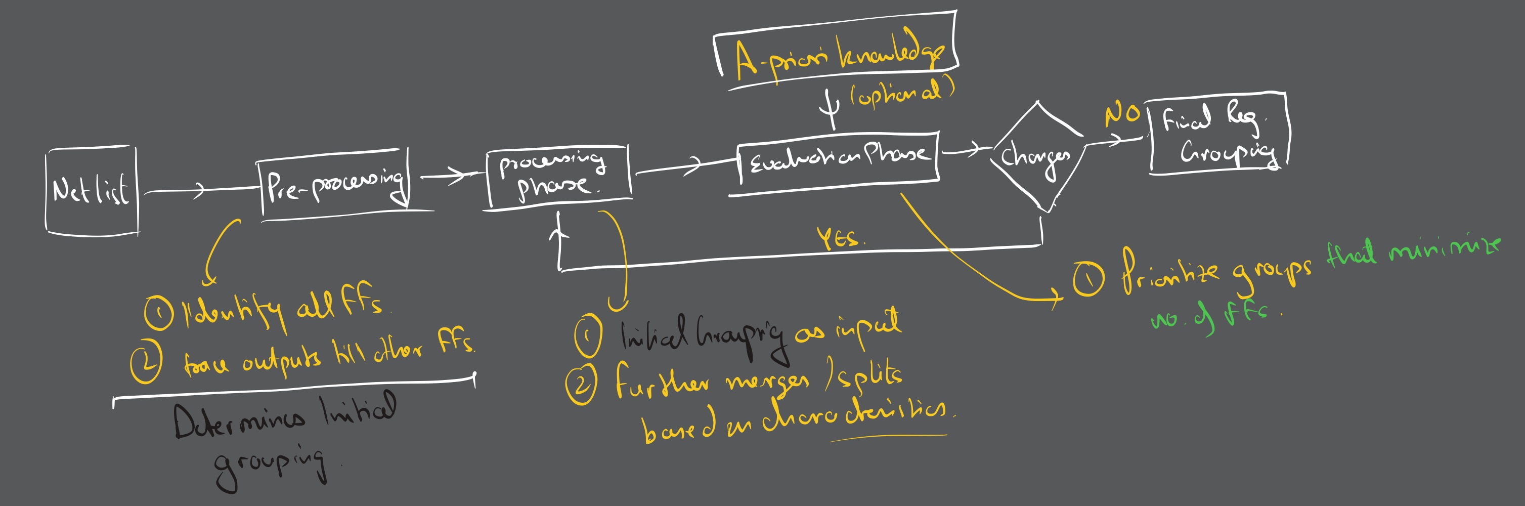

The goal is to reduce the netlist to registers + logic only. To do that, the paper employs three stages, which we’ll discuss now.

# Pre-Processing

Here we try to group the FFs into different initial stages. The premise of this phase is that

All successors/predecessors of a FF belong in the same stage

To achieve this, there is a 3 part process:

1. Forward and backward stage assignment
2. Result splitting
3. Final Merging

Before we move forward, let me set up the diagrams so that its easy to follow along. Let’s say that the FF netlist looks like this: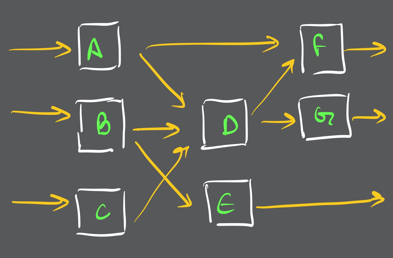

Note:

1. This is completely stripped of logic gates. Every node is a FF and every edge says that “there are no FFs in between these two FFs”

2. The FFs A, B and C are recieving primary inputs (i.e., from another source != FF). The FFs F and G are going to primary outputs (i.e., not to another FF).

3. Our analysis will focus on the interconnections between these and not primary inputs and outputs.

4. We will independently do the forward and backward stage assignments and only merge them in the end.

# Forward pass 1

Let’s start with the forward stage assignment. This follows a very simple rule:

For each FF, all of its successors belong in one stage together

Let’s write out the successors for each FF (ignoring primary input and outputs)

$$ \begin{aligned} \text{succ}(A) &= \lbrace D, F \rbrace \\ \text{succ}(B) &= \lbrace D, E \rbrace \\ \text{succ}(C) &= \lbrace D, E \rbrace \\ \text{succ}(D) &= \lbrace F, G \rbrace \end{aligned} $$

According to the rule, we will have to take a union of all the successor sets to get the set of all successors that belong in a single stage. That is,

$$ \text{succ}(A) \cup \text{succ}(B) \cup \text{succ}(C) \cup \text{succ}(D) = \lbrace D, F, G, E \rbrace $$

Thus the groups D, F, G and E must be of the same color according to the forward pass. So, we have this: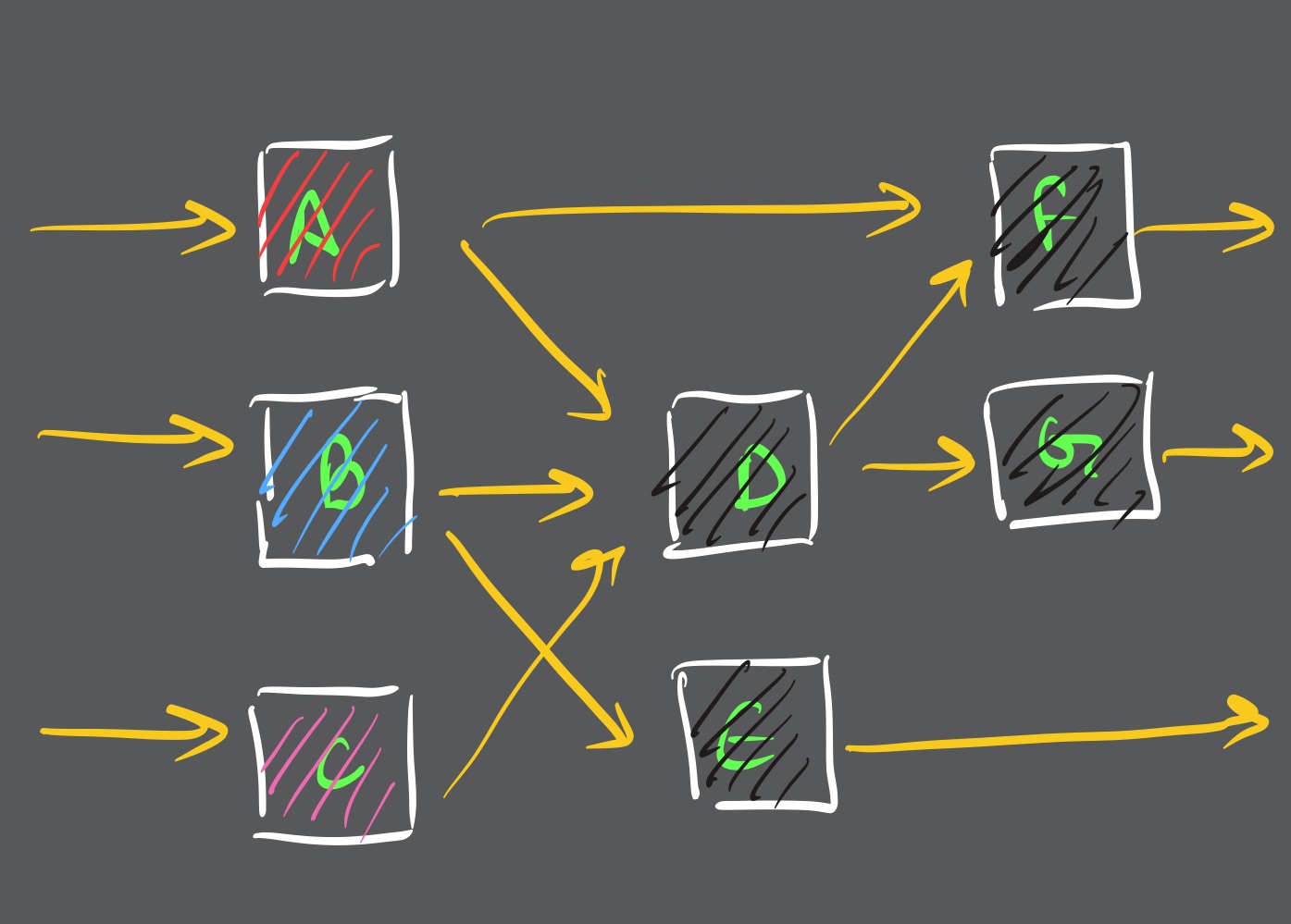

I have colored them black, while A, B and C are all different stages, hence colored differently.

# Backward pass 1

We’ll also do a backward stage assignment on the same initial diagram as mentioned before. This time the rule is:

For each FF, all of its predecessors belong in one stage together

Let’s write out the predecessors for each FF (ignoring primary input and outputs)

$$ \begin{aligned} \text{pred}(D) &= \lbrace A, B, C \rbrace \\ \text{pred}(E) &= \lbrace B, C \rbrace \\ \text{pred}(F) &= \lbrace A, D \rbrace \\ \text{pred}(G) &= \lbrace D \rbrace \end{aligned} $$

According to the rule, we will have to take a union of all the predecessor sets to get the set of all predecessors that belong in a single stage. That is,

$$ \text{pred}(D) \cup \text{pred}(E) \cup \text{pred}(F) \cup \text{pred}(G) = \lbrace A, B, C, D \rbrace $$

Thus the groups A, B, C and D must be of the same color according to the backward pass. So, we have this: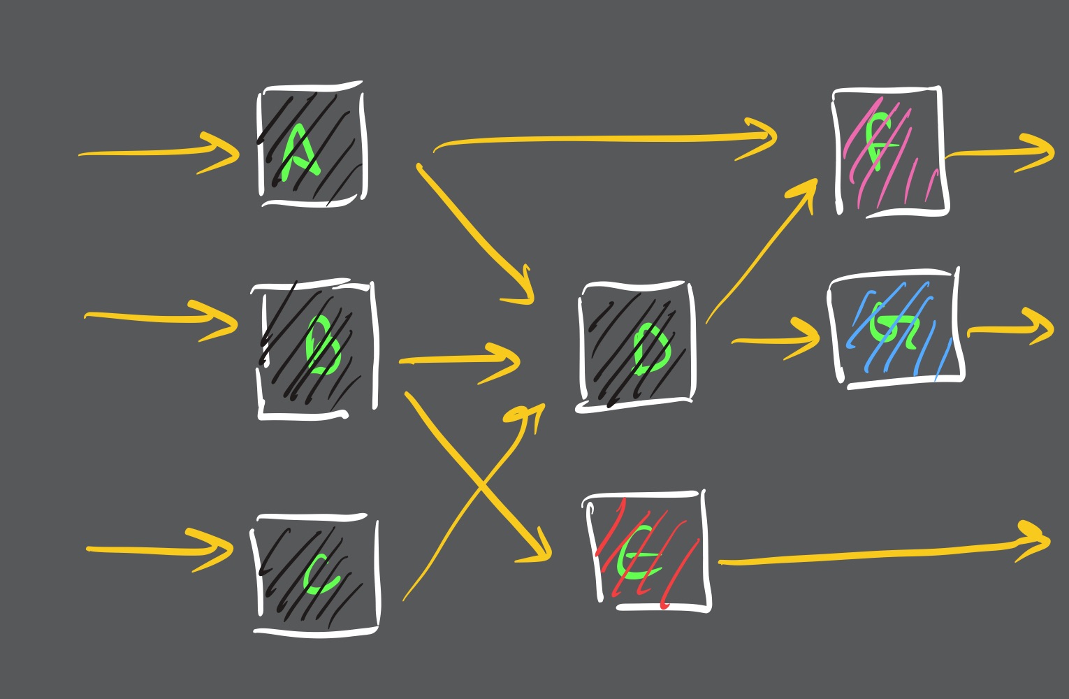

I have colored them black, while E, F and G are all different stages, hence colored differently.

# Forward pass 2 - Result splitting

The next rule says:

No FF in a stage may drive another FF in that stage

Recall that for the forward cycle we had D, F, G and E colored black and A, B and C colored differently. If we look at the diagram again, we can see that F and G are both driven by D.

This is a violation of the rule. To fix this, we’ll have to color F and G differently to ensure that they are part of a different group. So, we get this: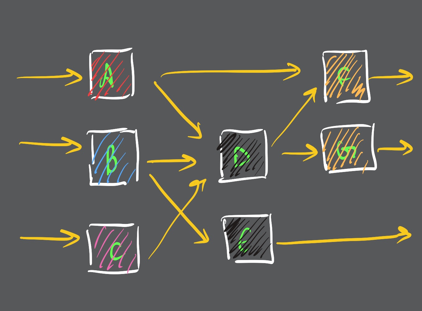

# Backward pass 2 - Result splitting

The same rule applies to the backward stage 2 as well. In this case, A, B and C are all driving D, thus they must be in mutually different groups.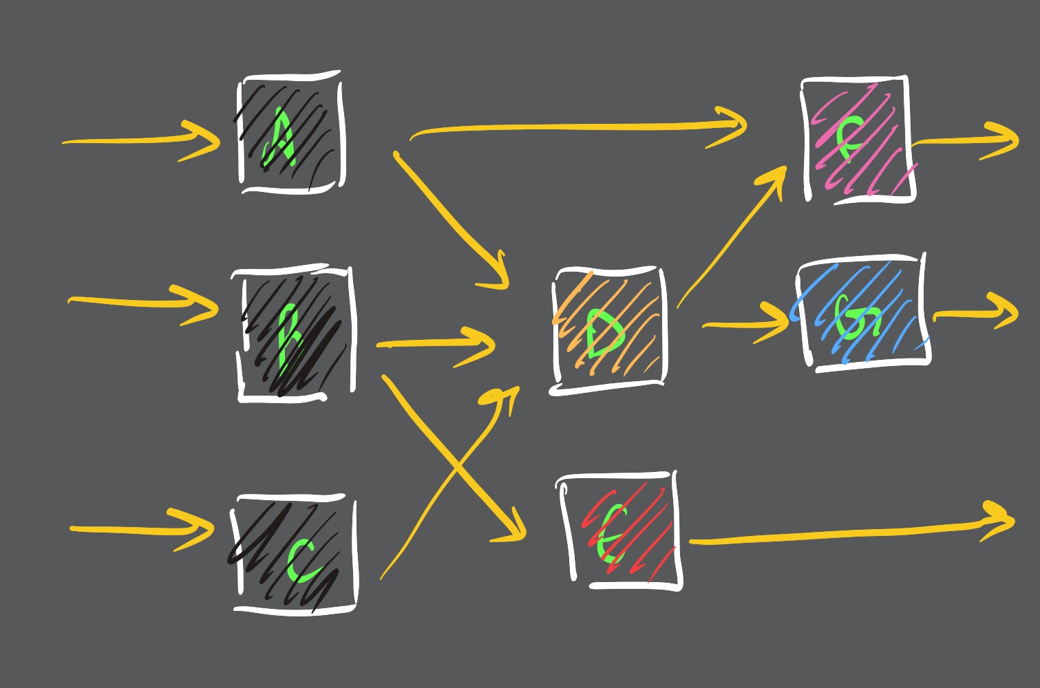

# Final merging

Now let’s first look at the groups that we already have:

$$ \begin{aligned} \text{forward} &= \lbrace A \rbrace; \lbrace B \rbrace; \lbrace C \rbrace; \lbrace D, E \rbrace; \lbrace F, G \rbrace \\ \text{backward} &= \lbrace A, B, C \rbrace; \lbrace D \rbrace; \lbrace E \rbrace; \lbrace F \rbrace; \lbrace G \rbrace \end{aligned} $$

The rule for merging the two stages together is:

Delete any stage that is a subset of another

In this case, stages $\lbrace A \rbrace$, $\lbrace B \rbrace$ and $\lbrace C \rbrace$ will be removed because they are subsets of $\lbrace A, B, C \rbrace$, similarly $\lbrace D \rbrace$ and $\lbrace E \rbrace$ will be removed as they are a subset of $\lbrace D, E \rbrace$, and $\lbrace F \rbrace$ and $\lbrace G \rbrace$ will be removed as they are a subset of $\lbrace F, G \rbrace$.

Now the final stages will look like:

$$ \text{final\_stage} = \lbrace A, B, C \rbrace; \lbrace D, E \rbrace; \lbrace F, G \rbrace $$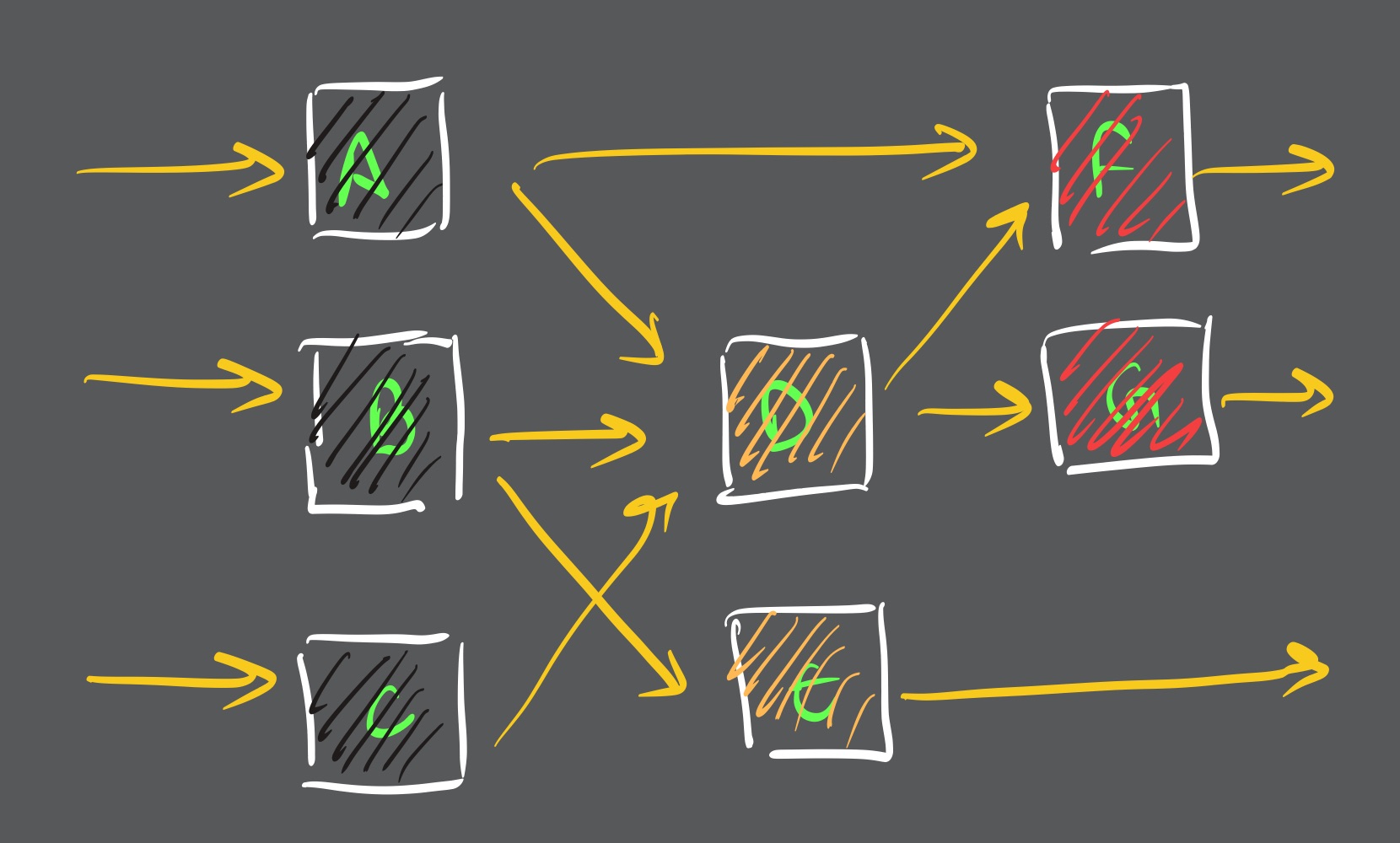

# Processing

Next up we have the processing step, which takes in as input the output of the pre-processing step (the different stages) and gives out a better grouping. This is done via a pair of 9 passes to the stages made above. These 9 passes listed out are:

1. Group by successor OR predecessor (2)
2. Iteratively group by successor OR predecessor (2)
3. Split by successor OR predecessor groups (2)
4. Group by number of sucessors OR predecessors (2)
5. Group by control signals (1)

Let’s first look at what each of them does.

# Group by successor OR predecessor

We already have stages that share same successor OR predecessor, in this case we’ll merge them. Consider this example for the predecessor merge (that is, merging cells which share the same predecessor)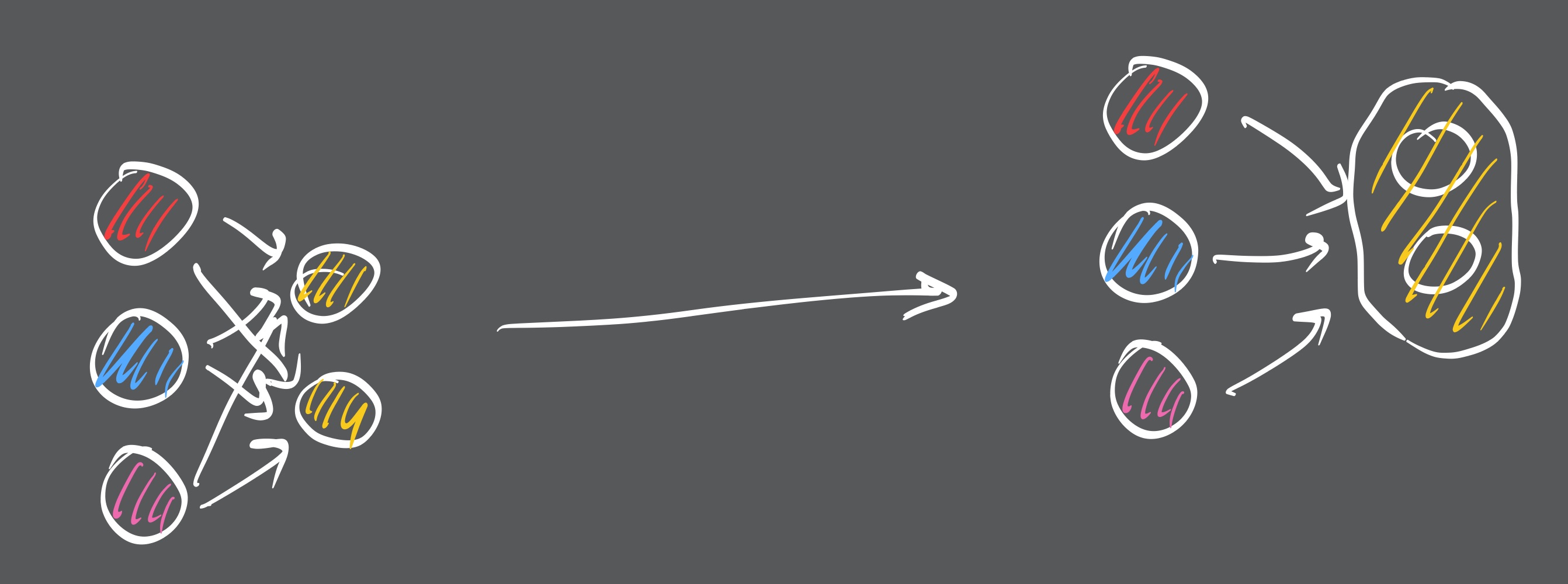

A similar procedure will follow for the successor.

# Iteratively group by successor OR predecessor

Exactly as above, but iteratively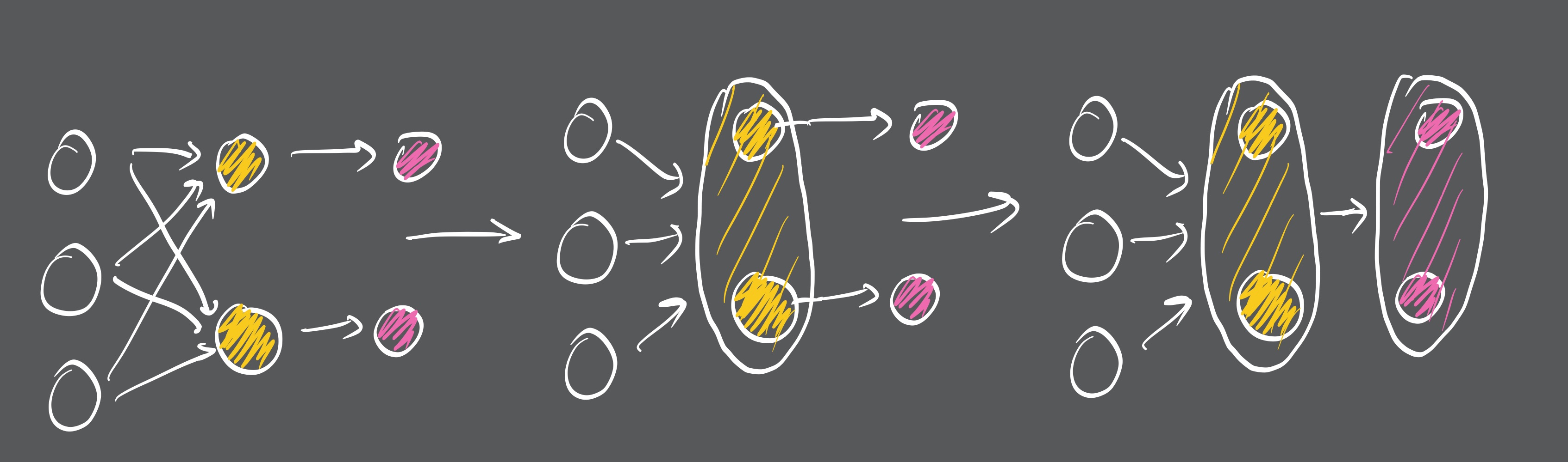

A similar procedure will follow for the successor.

# Split by successor OR predecessor groups

In this case, the successors or the predecessors of a group are analyzed. If for example, a few elements of a group have a successor X1 while the others have X2 then the group is split based on that.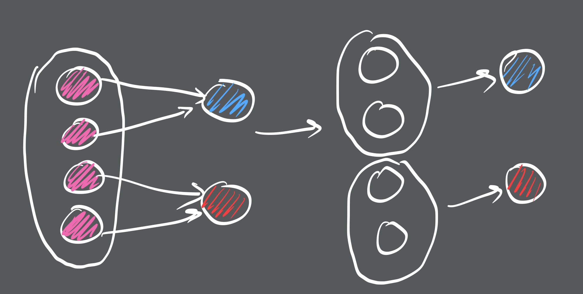

A similar procedure will follow for the predecessor.

# Group by number of sucessors OR predecessors

Here for each group we compute the maximum and minimum number of FF-successors/predecessors over all contained FFs. It then merges groups with matching values. Note that the rule check still ensures that no unrelated groups are merged.

This means, say you have a group with 4 FFs

$$ G = \lbrace A, B, C, D \rbrace $$

For each FF of each group we’ll compute the successor or predecessor, and based on the minimum and maximum we get there, we’ll assign a pair (min, max) to the group.

Then we’ll do this for all the groups, and merge the groups which have the same pair of (min, max).

# Group by control signals

This pass is to merge the groups with same clock and control signals.

# Voting mechanics

Now the thing is, we don’t do all 9 of them, we do only a pair. We can pick a pair, and permute them in any order (this makes the total possible options $9 \times 9 = 81$). We’ll be doing that for all these 81 possible pairs. So, we’ll have 81 possible “final” answers.

Now we need to pick the best one, which is where the voting idea comes into picture. The voting mechanism goes like this:

1. Count the occurence of each group in the final output across all 81 answers.
2. This frequency of each group is their vote.

Votes = how many of the 81 runs independently produced that exact set of flops.

To assemble the final answer then, we need to sort by the votes first and pick the winner.

There is a small quirk here. If the top n votes lie within 10% of the top, then we’ll pick all of them as tied canditates. Among the tied candidates now, we’ll choose the one which strands the fewest flops.

For example, say the following groups exist (among a set of only 6 FFs):

$$ \begin{aligned} G_{1} &= \lbrace 1, 2, 3, 4 \rbrace \\ G_{2} &= \lbrace 1, 2, 3, 4, 5, 6 \rbrace \end{aligned} $$

Let’s say that the frequency of $G_{1}$ was 74 and $G_{2}$ was 70. This is within 10% hence these are tied. Now, if we choose $G_{1}$ as the winner we’ll have $\lbrace 5, 6 \rbrace$ as a stranded group. But if we choose $G_{2}$ as the winner, we’ll have no stranded flops. Hence, we’ll pick $G_{2}$.

So, we’ll pick a winner and commit to it.

3. Once we have a winner, we’ll delete remaining candidate that overlaps it, since a flop can only belong to one register.

4. Repeat. Anything left unassigned becomes its own 1-flop group.

And that’s how we do DANA

Thanks for reading! Have a good day.