Exploratory math - Hermite polynomials
Contents:
# Introduction
A few days ago my brother asked me for the integral of $e^{-x^2}$, I told him that no closed form solution exists, and then got into some thinking. Meanwhile there was a typo on his end, and the problem he wanted to solve was the indefinite integral of $xe^{-x^2}$ which is trivial, so he was happy.
I started thinking because I wanted to understand the reason for the non-existence of closed form solutions. If you look at the graph of $f(t)=\int_0^t e^{-x^2} dx$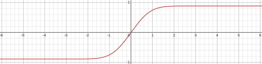
It looks so tantalizingly close to sigmoids, or tanhx or any other activation function we end up using in NNs! So, I was thinking even if no closed form solutions exist, why can’t we come up with an accurate approximation?
# TL;DR
TLDR;
I had not searched for anything prior to starting my work on this. Which means I did not know that a lot of smart people have figured out a lot of smart stuff in this area. I also did not end up deriving Winitzki Approximation or any other closed form approximation because I quickly digressed towards the gauss-hermite quadrature areas, starting from Hermite polynomials, deriving the recurrence relations and then moving up from there.
This is part one of the blog, which dives into hermite polynomials and the recurrence relation derivation only.
# Approach
My thought process went something like
Find constraints that the approximation should satisfy, an arbitrary number of constraints for an arbitrary degree of approximation
I was coming from a physics background, where for example you can apply the symmetries of the Galilean group to reduce a lagrangian into obeying Newton’s first law and prove
$$ \mathcal{L} = av^{2} $$
From this perspective it seemed ideal that I can zero in on the right nature of the approximation function by applying constraints to the world of functions. So, that’s what I tried.
Looking at the graph again, and this integral
$$ \int_0^{\infty} e^{-x^2} dx = \frac{\sqrt{\pi}}{2} $$
we can quickly define the following constraints in the least. Assume that the approximation function is $f(x)$:
The limits to infinity
$$ \lim_{x\to\infty} f(x) = \frac{\sqrt{\pi}}{2} $$
and,
$$ \lim_{x\to-\infty} f(x) = -\frac{\sqrt{\pi}}{2} $$
The value at 0
$$ f(0)=0 $$
We can use the fundamental theorem of calculus:
$$ \frac{d}{dt}\int_{0}^tf(x)dx = f(t) $$
to find $f'(0)$ as
$$ f'(0)=\left[ \frac{d}{dt}\int_0^te^{-x^2}dx \right\rvert_{x=0} = \left[e^{-x^2}\right\rvert_{x=0}=1 $$
Now these are good, but they are only three and I want an arbitrary number of constraints, which I can keep increasing to do better and better approximations. The idea I employed is to use higher order derivatives at 0.
I did a few by hand, and I will just write them down here so that you can see too:
$$ f'(t)=e^{-t^2}; \rvert_{t=0} = 1 $$
$$ f''(t)=-2te^{-t^2}; \rvert_{t=0} = 0 $$
$$ f'''(t)=(-2+4t^2)e^{-t^2}; \rvert_{t=0} = -2 $$
$$ f^{IV}(t)=(12t-8t^3)e^{-t^2}; \rvert_{t=0} = 0 $$
$$ f^{V}(t)=(12-48t^2+16t^4)e^{-t^2}; \rvert_{t=0} =12 $$
$$ f^{VI}(t)=(-120t+160t^3-32t^5)e^{-t^2}; \rvert_{t=0} = 0 $$
And so on. Now I cannot make a sense of the pattern here (at least not entirely) so I am going to write the coefficients down as a matrix.
The columns will be the coefficients of $x^0$, $x^1$, $x^2$…, while the rows will be for $f'$, $f''$… This is what the matrix ends up looking like:
$$ \def\arraystretch{1.3} \begin{array}{r|rrrrrrrr} & x^0 & x^1 & x^2 & x^3 & x^4 & x^5 & x^6 & x^7 \cr \hline f & 1 & 0 & 0 & 0 & 0 & 0 & 0 & 0 \cr f' & 0 & -2 & 0 & 0 & 0 & 0 & 0 & 0 \cr f'' & -2 & 0 & 4 & 0 & 0 & 0 & 0 & 0 \cr f''' & 0 & 12 & 0 & -8 & 0 & 0 & 0 & 0 \cr f^{(IV)} & 12 & 0 & -48 & 0 & 16 & 0 & 0 & 0 \cr f^{(V)} & 0 & -120 & 0 & 160 & 0 & -32 & 0 & 0 \cr f^{(VI)} & -120 & 0 & 720 & 0 & -480 & 0 & 64 & 0 \cr f^{(VII)} & 0 & 1680 & 0 & -3360 & 0 & 1344 & 0 & -128 \end{array} $$
I computed a few more rows to see the pattern clearly
A few observations:
- The matrix is lower triangular
- The diagonal elements form a geometric progression with $a=1; r=-2$
- All alternate elements of the matrix are 0
What we need is a way to generate any row of this matrix. Because if we have that, then we can arbitrarily have our approximation satisfy the Nth derivative of the original function at 0.
Let $A$ be a $N\times N$ matrix with elements $a_{i,j}$. Then the following relations should hold (based purely on observations so far):
- $a_{i,j} = 0; \forall i < j$ - Handles the lower triangular bit
- $a_{i,i} = (-2)^{i-1}; 1 \le i \le N$ - Handles the diagonal elements
- $a_{i, i-2k+1} = 0; \forall i > 1; k \le \frac{i}{2}$ - Handles the alternating zeroes
- $a_{i,1} = a_{i-1, 2} \forall i$
The fourth relation says that the second column shifted down is the first column.
Awesome, but we still need the others. I took me a while to figure out the relationship, let’s say about an hour of staring and trying out different combinations, but eventually this is what I had
$$ \def\arraystretch{1.5} \begin{array}{r|rrrrrrrr} & x^0 & x^1 & x^2 & x^3 & x^4 & x^5 & x^6 & x^7 \cr \hline f & \textcolor{#D4A017}{1} & 0 & 0 & 0 & 0 & 0 & 0 & 0 \cr f' & 0 & \textcolor{#D4A017}{-2} & 0 & 0 & 0 & 0 & 0 & 0 \cr f'' & \textcolor{#E03131}{-2} & 0 & \textcolor{#D4A017}{4} & 0 & 0 & 0 & 0 & 0 \cr f''' & 0 & \textcolor{#E03131}{12} & 0 & \textcolor{#D4A017}{-8} & 0 & 0 & 0 & 0 \cr f^{(IV)} & \textcolor{#E95496}{12} & 0 & \textcolor{#E03131}{-48} & 0 & \textcolor{#D4A017}{16} & 0 & 0 & 0 \cr f^{(V)} & 0 & \textcolor{#E95496}{-120} & 0 & \textcolor{#E03131}{160} & 0 & \textcolor{#D4A017}{-32} & 0 & 0 \cr f^{(VI)} & \textcolor{#4C9BE8}{-120} & 0 & \textcolor{#E95496}{720} & 0 & \textcolor{#E03131}{-480} & 0 & \textcolor{#D4A017}{64} & 0 \cr f^{(VII)} & 0 & \textcolor{#4C9BE8}{1680} & 0 & \textcolor{#E95496}{-3360} & 0 & \textcolor{#E03131}{1344} & 0 & \textcolor{#D4A017}{-128} \end{array} $$
(the arrows I drew on paper can’t be drawn here, so instead every entry is coloured by the hop that lands on it: gold is the diagonal, and each coloured entry is the target of an arrow of that colour)
It was quite complicated to have this rendered in latex! Anyway, each arrow is a ratio between two entries in the same row, two columns apart. The numerators are always the triangular numbers 1, 3, 6, 10, …; the denominator is fixed per colour and says which hop you’re on.
| Colour | Hop | Denominator | Ratios, starting from row… |
|---|---|---|---|
| Red | diagonal → 2 left | 2 | $\tfrac12, \tfrac32, \tfrac62, \tfrac{10}2, \ldots$ from row 3 |
| Pink | 2 left → 4 left | 4 | $\tfrac14, \tfrac34, \tfrac64, \ldots$ from row 5 |
| Blue | 4 left → 6 left | 6 | $\tfrac16, \tfrac36, \ldots$ from row 7 |
Each coloured family of arrows moves two columns left within a row. Every colour shares the same numerators -> the triangular numbers 1, 3, 6, 10, …; and differs only in its denominator: 2 for the first hop, 4 for the second, 6 for the third. The three colours are the same pattern at successive distances from the diagonal.
Note that the numbers 1, 3, 6, 10 are consecutive sums, so we can use the $n(n+1)/2$ formula for them!
Well, now its not too hard to see that the following pops up:
$$ a_{i,i-2} = a_{i,i} \left( \frac{(i-2)(i-1)}{2\cdot2} \right); \forall i>2 $$
and,
$$ a_{i,i-4} = a_{i,i} \left( \frac{(i-2)(i-1)}{2\cdot2} \right) \left( \frac{(i-4)(i-3)}{2\cdot4} \right); \forall i>4 $$
and,
$$ a_{i,i-6} = a_{i,i} \left( \frac{(i-2)(i-1)}{2\cdot2} \right) \left( \frac{(i-4)(i-3)}{2\cdot4} \right)\left( \frac{(i-6)(i-5)}{2\cdot6} \right); \forall i>6 $$
So we can write the general formula as
$$ a_{i,i-w} = a_{i,i} \prod_{k=1}^w(i-k) \left( \frac{(-1)^{w/2}}{2^w\left(\frac{w}{2}\right)!}\right); \forall i > w; w \in \lbrace 2,4,6,\ldots \rbrace $$
And we can substitute the value for $a_{i,i}$ in there,
$$ a_{i,i-w} = (-2)^{i-1} \prod_{k=1}^w(i-k) \left( \frac{(-1)^{w/2}}{2^w\left(\frac{w}{2}\right)!}\right); \forall i > w; w \in \lbrace 2,4,6,\ldots \rbrace $$
And that gives us all the values in the matrix! Since our goal was to compute $f^{i}(0)$ we can substitute in $x=0$ for this relation here to get:
$$ f^{i}(0) = \begin{cases} 0 & \text{if } i \text{ is even} \cr \frac{(-1)^\psi}{\psi!} \prod_{k=1}^{2\psi}(2\psi+1-k) & \text{if } i = 2\psi+1 \text{ where }\psi\in N \end{cases} $$
Now we have the 5 constraints which we can use to arbitrarily approximate the gaussian integral.